
Analyze a query plan
Learn how to read and analyze a query plan to understand query execution steps and data organization, and find performance bottlenecks.
When you query InfluxDB v3, the Querier devises a query plan for executing the query. The engine tries to determine the optimal plan for the query structure and data. By learning how to generate and interpret reports for the query plan, you can better understand how the query is executed and identify bottlenecks that affect the performance of your query.
For example, if the query plan reveals that your query reads a large number of Parquet files, you can then take steps to optimize your query, such as add filters to read less data or configure your cluster to store fewer and larger files.
- Use EXPLAIN keywords to view a query plan
- Read an EXPLAIN report
- Read a query plan
- Analyze a query plan for leading edge data
Use EXPLAIN keywords to view a query plan
Use the EXPLAIN keyword (and the optional ANALYZE and VERBOSE keywords) to view the query plans for a query.
Read an EXPLAIN report
When you use EXPLAIN keywords to view a query plan, the report contains the following:
- two columns:
plan_typeandplan - one row for the logical plan (
logical_plan) - one row for the physical plan (
physical_plan)
Read a query plan
Plans are in tree format–each plan is an upside-down tree in which execution and data flow from leaf nodes, the innermost steps in the plan, to outer branch nodes. Whether reading a logical or physical plan, keep the following in mind:
- Start at the leaf nodes and read upward.
- At the top of the plan, the root node represents the final, encompassing step.
In a physical plan, each step is an ExecutionPlan node that receives expressions for input data and output requirements, and computes a partition of data.
Use the following steps to analyze a query plan and estimate how much work is required to complete the query. The same steps apply regardless of how large or complex the plan might seem.
- Start from the furthest indented steps (the leaf nodes), and read upward.
- Understand the job of each
ExecutionPlannode–for example, aUnionExecnode encompassing the leaf nodes means that theUnionExecconcatenates the output of all the leaves. - For each expression, answer the following questions:
- What is the shape and size of data input to the plan?
- What is the shape and size of data output from the plan?
The remainder of this guide walks you through analyzing a physical plan. Understanding the sequence, role, input, and output of nodes in your query plan can help you estimate the overall workload and find potential bottlenecks in the query.
Example physical plan for a SELECT - ORDER BY query
The following example shows how to read an EXPLAIN report and a physical query plan.
Given h20 measurement data and the following query:
EXPLAIN SELECT city, min_temp, time FROM h2o ORDER BY city ASC, time DESC;
The output is similar to the following:
EXPLAIN report
| plan_type     | plan                                                                     |
+---------------+--------------------------------------------------------------------------+
| logical_plan  | Sort: h2o.city ASC NULLS LAST, h2o.time DESC NULLS FIRST                 |
|               |   TableScan: h2o projection=[city, min_temp, time]                       |
| physical_plan | SortPreservingMergeExec: [city@0 ASC NULLS LAST,time@2 DESC]             |
|               |   UnionExec                                                              |
|               |     SortExec: expr=[city@0 ASC NULLS LAST,time@2 DESC]                   |
|               |       ParquetExec: file_groups={...}, projection=[city, min_temp, time]  |
|               |     SortExec: expr=[city@0 ASC NULLS LAST,time@2 DESC]                   |
|               |       ParquetExec: file_groups={...}, projection=[city, min_temp, time]  |
|               |                                                                          |
Output from EXPLAIN SELECT city, min_temp, time FROM h2o ORDER BY city ASC, time DESC;
Each step, or node, in the physical plan is an ExecutionPlan name and the key-value expressions that contain relevant parts of the query–for example, the first node in the EXPLAIN report physical plan is a ParquetExec execution plan:
ParquetExec: file_groups={...}, projection=[city, min_temp, time]
Because ParquetExec and RecordBatchesExec nodes retrieve and scan data in InfluxDB queries, every query plan starts with one or more of these nodes.
Physical plan data flow
Data flows up in a query plan.
The following diagram shows the data flow and sequence of nodes in the EXPLAIN report physical plan:
SortPreservingMergeExec
UnionExec
SortExec
ParquetExec
SortExec
ParquetExec
Execution and data flow in the EXPLAIN report physical plan.
ParquetExec nodes execute in parallel and UnionExec combines their output.
The following steps summarize the physical plan execution and data flow:
- Two
ParquetExecplans, in parallel, read data from Parquet files:- Each
ParquetExecnode processes one or more file groups. - Each file group contains one or more Parquet file paths.
- A
ParquetExecnode processes its groups in parallel, reading each group’s files sequentially. - The output is a stream of data to the corresponding
SortExecnode.
- Each
- The
SortExecnodes, in parallel, sort the data bycity(ascending) andtime(descending). Sorting is required by theSortPreservingMergeExecplan. - The
UnionExecnode concatenates the streams to union the output of the parallelSortExecnodes. - The
SortPreservingMergeExecnode merges the previously sorted and unioned data fromUnionExec.
Example EXPLAIN report for an empty result set
If your table doesn’t contain data for the time range in your query, the physical plan starts with an EmptyExec leaf node–for example:
ProjectionExec: expr=[temp@0 as temp]
    SortExec: expr=[time@1 ASC NULLS LAST]
        EmptyExec: produce_one_row=false
Analyze a query plan for leading edge data
The following sections guide you through analyzing a physical query plan for a typical time series use case–aggregating recently written (leading edge) data.
Although the query and plan are more complex than in the preceding example, you’ll follow the same steps to read the query plan.
After learning how to read the query plan, you’ll have an understanding of ExecutionPlans, data flow, and potential query bottlenecks.
Sample data
Consider the following h20 data, represented as “chunks” of line protocol, written to InfluxDB:
// h20 data
// The following data represents 5 batches, or "chunks", of line protocol
// written to InfluxDB.
// - Chunks 1-4 are ingested and each is persisted to a separate partition file in storage.
// - Chunk 5 is ingested and not yet persisted to storage.
// - Chunks 1 and 2 cover short windows of time that don't overlap times in other chunks.
// - Chunks 3 and 4 cover larger windows of time and the time ranges overlap each other.
// - Chunk 5 contains the largest time range and overlaps with chunk 4, the Parquet file with the largest time-range.
// - In InfluxDB, a chunk never duplicates its own data.
//
// Chunk 1: stored Parquet file
// - time range: 50-249
// - no duplicates in its own chunk
// - no overlap with any other chunks
[
"h2o,state=MA,city=Bedford min_temp=71.59 150",
"h2o,state=MA,city=Boston min_temp=70.4, 50",
"h2o,state=MA,city=Andover max_temp=69.2, 249",
],

// Chunk 2: stored Parquet file
// - time range: 250-349
// - no duplicates in its own chunk
// - no overlap with any other chunks
// - adds a new field (area)
[
"h2o,state=CA,city=SF min_temp=79.0,max_temp=87.2,area=500u 300",
"h2o,state=CA,city=SJ min_temp=75.5,max_temp=84.08 349",
"h2o,state=MA,city=Bedford max_temp=78.75,area=742u 300",
"h2o,state=MA,city=Boston min_temp=65.4 250",
],

// Chunk 3: stored Parquet file
// - time range: 350-500
// - no duplicates in its own chunk
// - overlaps chunk 4
[
"h2o,state=CA,city=SJ min_temp=77.0,max_temp=90.7 450",
"h2o,state=CA,city=SJ min_temp=69.5,max_temp=88.2 500",
"h2o,state=MA,city=Boston min_temp=68.4 350",
],

// Chunk 4: stored Parquet file
// - time range: 400-600
// - no duplicates in its own chunk
// - overlaps chunk 3
[
 "h2o,state=CA,city=SF min_temp=68.4,max_temp=85.7,area=500u 600",
 "h2o,state=CA,city=SJ min_temp=69.5,max_temp=89.2 600",  // duplicates row 3 in chunk 5
 "h2o,state=MA,city=Bedford max_temp=80.75,area=742u 400", // overlaps chunk 3
 "h2o,state=MA,city=Boston min_temp=65.40,max_temp=82.67 400", // overlaps chunk 3
],

// Chunk 5: Ingester data
// - time range: 550-700
// - overlaps and duplicates data in chunk 4
[
"h2o,state=MA,city=Bedford max_temp=88.75,area=742u 600", // overlaps chunk 4
"h2o,state=CA,city=SF min_temp=68.4,max_temp=85.7,area=500u 650",
"h2o,state=CA,city=SJ min_temp=68.5,max_temp=90.0 600", // duplicates row 2 in chunk 4
"h2o,state=CA,city=SJ min_temp=75.5,max_temp=84.08 700",
"h2o,state=MA,city=Boston min_temp=67.4 550", // overlaps chunk 4
]
The following query selects all the data:
SELECT state, city, min_temp, max_temp, area, time
FROM h2o
ORDER BY state asc, city asc, time desc;
The output is the following:
+-------+---------+----------+----------+------+--------------------------------+
| state | city    | min_temp | max_temp | area | time                           |
+-------+---------+----------+----------+------+--------------------------------+
| CA    | SF      | 68.4     | 85.7     | 500  | 1970-01-01T00:00:00.000000650Z |
| CA    | SF      | 68.4     | 85.7     | 500  | 1970-01-01T00:00:00.000000600Z |
| CA    | SF      | 79.0     | 87.2     | 500  | 1970-01-01T00:00:00.000000300Z |
| CA    | SJ      | 75.5     | 84.08    |      | 1970-01-01T00:00:00.000000700Z |
| CA    | SJ      | 68.5     | 90.0     |      | 1970-01-01T00:00:00.000000600Z |
| CA    | SJ      | 69.5     | 88.2     |      | 1970-01-01T00:00:00.000000500Z |
| CA    | SJ      | 77.0     | 90.7     |      | 1970-01-01T00:00:00.000000450Z |
| CA    | SJ      | 75.5     | 84.08    |      | 1970-01-01T00:00:00.000000349Z |
| MA    | Andover |          | 69.2     |      | 1970-01-01T00:00:00.000000249Z |
| MA    | Bedford |          | 88.75    | 742  | 1970-01-01T00:00:00.000000600Z |
| MA    | Bedford |          | 80.75    | 742  | 1970-01-01T00:00:00.000000400Z |
| MA    | Bedford |          | 78.75    | 742  | 1970-01-01T00:00:00.000000300Z |
| MA    | Bedford | 71.59    |          |      | 1970-01-01T00:00:00.000000150Z |
| MA    | Boston  | 67.4     |          |      | 1970-01-01T00:00:00.000000550Z |
| MA    | Boston  | 65.4     | 82.67    |      | 1970-01-01T00:00:00.000000400Z |
| MA    | Boston  | 68.4     |          |      | 1970-01-01T00:00:00.000000350Z |
| MA    | Boston  | 65.4     |          |      | 1970-01-01T00:00:00.000000250Z |
| MA    | Boston  | 70.4     |          |      | 1970-01-01T00:00:00.000000050Z |
+-------+---------+----------+----------+------+--------------------------------+
Sample query
The following query selects leading edge data from the sample data:
SELECT city, count(1)
FROM h2o
WHERE time >= to_timestamp(200) AND time < to_timestamp(700)
  AND state = 'MA'
GROUP BY city
ORDER BY city ASC;
The output is the following:
+---------+-----------------+
| city    | COUNT(Int64(1)) |
+---------+-----------------+
| Andover | 1               |
| Bedford | 3               |
| Boston  | 4               |
+---------+-----------------+
EXPLAIN report for the leading edge data query
The following query generates the EXPLAIN report for the preceding sample query:
EXPLAIN SELECT city, count(1)
FROM h2o
WHERE time >= to_timestamp(200) AND time < to_timestamp(700)
  AND state = 'MA'
GROUP BY city
ORDER BY city ASC;
The comments in the sample data tell you which data chunks overlap or duplicate data in other chunks. Two chunks of data overlap if there are portions of time for which data exists in both chunks. You’ll learn how to recognize overlapping and duplicate data in a query plan later in this guide.
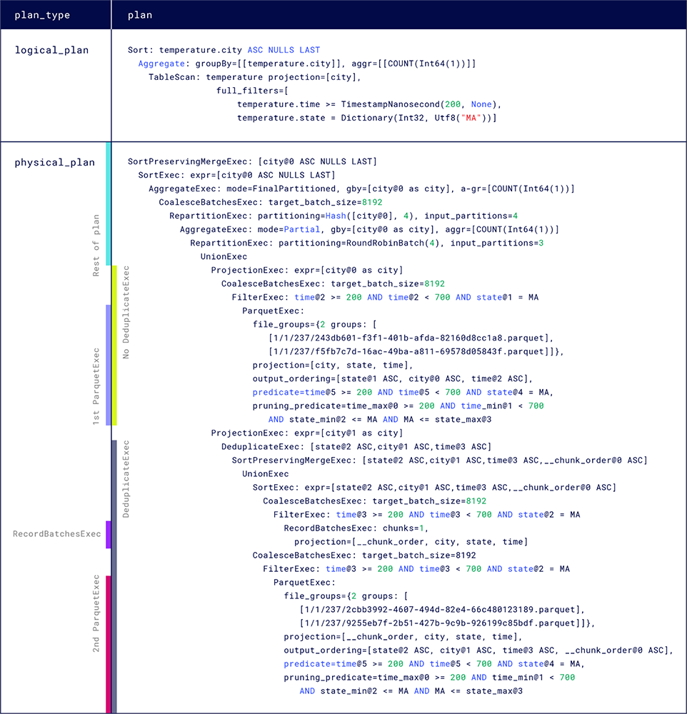
Unlike the sample data, your data likely doesn’t tell you where overlaps or duplicates exist. A physical plan can reveal overlaps and duplicates in your data and how they affect your queries–for example, after learning how to read a physical plan, you might summarize the data scanning steps as follows:
- Query execution starts with two
ParquetExecand oneRecordBatchesExecexecution plans that run in parallel. - The first
ParquetExecnode reads two files that don’t overlap any other files and don’t duplicate data; the files don’t require deduplication. - The second
ParquetExecnode reads two files that overlap each other and overlap the ingested data scanned in theRecordBatchesExecnode; the query plan must include the deduplication process for these nodes before completing the query.
The remaining sections analyze ExecutionPlan node structure and arguments in the example physical plan.
The example includes DataFusion and InfluxDB-specific ExecutionPlan nodes.
Locate the physical plan
To begin analyzing the physical plan for the query, find the row in the EXPLAIN report where the plan_type column has the value physical_plan.
The plan column for the row contains the physical plan.
Read the physical plan
The following sections follow the steps to read a query plan and examine the physical plan nodes and their input and output.
To read the execution flow of a query plan, always start from the innermost (leaf) nodes and read up toward the top outermost root node.
Physical plan leaf nodes
Leaf node structures in the physical plan
Data scanning nodes (ParquetExec and RecordBatchesExec)
The example physical plan contains three leaf nodes–the innermost nodes where the execution flow begins:
ParquetExecnodes retrieve and scan data from Parquet files in the Object store- a
RecordBatchesExecnode retrieves recently written, yet-to-be-persisted data from the Ingester
Because ParquetExec and RecordBatchesExec retrieve and scan data for a query, every query plan starts with one or more of these nodes.
The number of ParquetExec and RecordBatchesExec nodes and their parameter values can tell you which data (and how much) is retrieved for your query, and how efficiently the plan handles the organization (for example, partitioning and deduplication) of your data.
For convenience, this guide uses the names ParquetExec_A and ParquetExec_B for the ParquetExec nodes in the example physical plan .
Reading from the top of the physical plan, ParquetExec_A is the first leaf node in the physical plan and ParquetExec_B is the last (bottom) leaf node.
The names indicate the nodes’ locations in the report, not their order of execution.
ParquetExec_A
ParquetExec: file_groups={2 groups: [[1/1/b862a7e9b329ee6a418cde191198eaeb1512753f19b87a81def2ae6c3d0ed237/243db601-f3f1-401b-afda-82160d8cc1a8.Parquet], [1/1/b862a7e9b329ee6a418cde191198eaeb1512753f19b87a81def2ae6c3d0ed237/f5fb7c7d-16ac-49ba-a811-69578d05843f.Parquet]]}, projection=[city, state, time], output_ordering=[state@1 ASC, city@0 ASC, time@2 ASC], predicate=time@5 >= 200 AND time@5 < 700 AND state@4 = MA, pruning_predicate=time_max@0 >= 200 AND time_min@1 < 700 AND state_min@2 <= MA AND MA <= state_max@3 |
ParquetExec_A, the first ParquetExec node
ParquetExec_A has the following traits:
file_groups
A file group is a list of files for the operator to read. Files are referenced by path:
1/1/b862a7e9b.../243db601-....parquet1/1/b862a7e9b.../f5fb7c7d-....parquet
The path structure represents how your data is organized. You can use the file paths to gather more information about the query–for example:
- to find file information (for example: size and number of rows) in the catalog
- to download the Parquet file from the Object store for debugging
- to find how many partitions the query reads
A path has the following structure:
<namespace_id>/<table_id>/<partition_hash_id>/<uuid_of_the_file>.Parquet
    1         /    1    /b862a7e9b329ee6a4.../243db601-f3f1-4....Parquet
namespace_id: the namespace (database) being queriedtable_id: the table (measurement) being queriedpartition_hash_id: the partition this file belongs to. You can count partition IDs to find how many partitions the query reads.uuid_of_the_file: the file identifier.
ParquetExec processes groups in parallel and reads the files in each group sequentially.
file_groups={2 groups: [[1/1/b862a7e9b329ee6a4/243db601....parquet], [1/1/b862a7e9b329ee6a4/f5fb7c7d....parquet]]}
{2 groups: [[file], [file]}: ParquetExec_A receives two groups with one file per group. Therefore, ParquetExec_A reads two files in parallel.
projection
projection lists the table columns for the ExecutionPlan to read and output.
projection=[city, state, time]
[city, state, time]: the sample data contains many columns, but the sample query requires the Querier to read only three
output_ordering
output_ordering specifies the sort order for the ExecutionPlan output.
The Query planner passes the parameter if the output should be ordered and if the planner knows the order.
output_ordering=[state@2 ASC, city@1 ASC, time@3 ASC, __chunk_order@0 ASC]
When storing data to Parquet files, InfluxDB sorts the data to improve storage compression and query efficiency and the planner tries to preserve that order for as long as possible.
Generally, the output_ordering value that ParquetExec receives is the ordering (or a subset of the ordering) of stored data.
By design, RecordBatchesExec data isn’t sorted.
In the example, the planner specifies that ParquetExec_A use the existing sort order state ASC, city ASC, time ASC, for output.
To view the sort order of your stored data, generate an EXPLAIN report for a SELECT ALL query–for example:
EXPLAIN SELECT * FROM TABLE_NAME WHERE time > now() - interval '1 hour'
Reduce the time range if the query returns too much data.
predicate
predicate is the data filter specified in the query.
predicate=time@5 >= 200 AND time@5 < 700 AND state@4 = MA
pruning predicate
pruning_predicate is created from the predicate value and is the predicate actually used for pruning data and files from the chosen partitions.
The default filters files by time.
pruning_predicate=time_max@0 >= 200 AND time_min@1 < 700 AND state_min@2 <= MA AND MA <= state_max@3
Before the physical plan is generated, an additional partition pruning step uses predicates on partitioning columns to prune partitions.
RecordBatchesExec
RecordBatchesExec: chunks=1, projection=[__chunk_order, city, state, time]
RecordBatchesExec is an InfluxDB-specific ExecutionPlan implementation that retrieves recently written, yet-to-be-persisted data from the Ingester.
In the example, RecordBatchesExec contains the following expressions:
chunks
chunks is the number of data chunks received from the Ingester.
chunks=1
chunks=1:RecordBatchesExecreceives one data chunk.
projection
The projection list specifies the columns or expressions for the node to read and output.
[__chunk_order, city, state, time]
__chunk_order: orders chunks and files for deduplicationcity, state, time: the same columns specified inParquetExec_A projection
The presence of __chunk_order in data scanning nodes indicates that data overlaps, and is possibly duplicated, among the nodes.
ParquetExec_B
The bottom leaf node in the example physical plan is another ParquetExec operator, ParquetExec_B.
ParquetExec_B expressions
ParquetExec:
  file_groups={2 groups: [[1/1/b862a7e9b.../2cbb3992-....Parquet],
   [1/1/b862a7e9b.../9255eb7f-....Parquet]]},
  projection=[__chunk_order, city, state, time],
  output_ordering=[state@2 ASC, city@1 ASC, time@3 ASC, __chunk_order@0 ASC],
  predicate=time@5 >= 200 AND time@5 < 700 AND state@4 = MA,
  pruning_predicate=time_max@0 >= 200 AND time_min@1 < 700 AND state_min@2 <= MA AND MA <= state_max@3
Because ParquetExec_B has overlaps, the projection and output_ordering expressions use the __chunk_order column used in RecordBatchesExec projection.
The presence of __chunk_order in data scanning nodes indicates that data overlaps, and is possibly duplicated, among the nodes.
The remaining ParquetExec_B expressions are similar to those in ParquetExec_A.
How a query plan distributes data for scanning
If you compare file_group paths in ParquetExec_A to those in ParquetExec_B, you’ll notice that both contain files from the same partition:
1/1/b862a7e9b329ee6a4.../...
The planner may distribute files from the same partition to different scan nodes for several reasons, including optimizations for handling overlaps–for example:
- to separate non-overlapped files from overlapped files to minimize work required for deduplication (which is the case in this example)
- to distribute non-overlapped files to increase parallel execution
Analyze branch structures
After data is output from a data scanning node, it flows up to the next parent (outer) node.
In the example plan:
- Each leaf node is the first step in a branch of nodes planned for processing the scanned data.
- The three branches execute in parallel.
- After the leaf node, each branch contains the following similar node structure:
...
CoalesceBatchesExec: target_batch_size=8192
    FilterExec: time@3 >= 200 AND time@3 < 700 AND state@2 = MA
    ...
FilterExec: time@3 >= 200 AND time@3 < 700 AND state@2 = MA: filters data for the conditiontime@3 >= 200 AND time@3 < 700 AND state@2 = MA, and guarantees that all data is pruned.CoalesceBatchesExec: target_batch_size=8192: combines small batches into larger batches. See the DataFusion [CoalesceBatchesExec] documentation.
Sorting yet-to-be-persisted data
In the RecordBatchesExec branch, the node that follows CoalesceBatchesExec is a SortExec node:
SortExec: expr=[state@2 ASC,city@1 ASC,time@3 ASC,__chunk_order@0 ASC]
The node uses the specified expression state ASC, city ASC, time ASC, __chunk_order ASC to sort the yet-to-be-persisted data.
Neither ParquetExec_A nor ParquetExec_B contain a similar node because data in the Object store is already sorted (by the Ingester or the Compactor) in the given order; the query plan only needs to sort data that arrives from the Ingester.
Recognize overlapping and duplicate data
In the example physical plan, the ParquetExec_B and RecordBatchesExec nodes share the following parent nodes:
...
DeduplicateExec: [state@2 ASC,city@1 ASC,time@3 ASC]
    SortPreservingMergeExec: [state@2 ASC,city@1 ASC,time@3 ASC,__chunk_order@0 ASC]
        UnionExec
            ...
UnionExec: unions multiple streams of input data by concatenating the partitions.UnionExecdoesn’t do any merging and is fast to execute.SortPreservingMergeExec: [state@2 ASC,city@1 ASC,time@3 ASC,__chunk_order@0 ASC]: merges already sorted data; indicates that preceding data (from nodes below it) is already sorted. The output data is a single sorted stream.DeduplicateExec: [state@2 ASC,city@1 ASC,time@3 ASC]: deduplicates an input stream of sorted data. BecauseSortPreservingMergeExecensures a single sorted stream, it often, but not always, precedesDeduplicateExec.
A DeduplicateExec node indicates that encompassed nodes have overlapped data–data in a file or batch have timestamps in the same range as data in another file or batch.
Due to how InfluxDB organizes data, data is never duplicated within a file.
In the example, the DeduplicateExec node encompasses ParquetExec_B and the RecordBatchesExec node, which indicates that ParquetExec_B file group files overlap the yet-to-be persisted data.
The following sample data excerpt shows overlapping data between a file and Ingester data:
// Chunk 4: stored Parquet file
//   - time range: 400-600
[
 "h2o,state=CA,city=SF min_temp=68.4,max_temp=85.7,area=500u 600",
],

// Chunk 5: Ingester data
//   - time range: 550-700
//   - overlaps and duplicates data in chunk 4
[
"h2o,state=MA,city=Bedford max_temp=88.75,area=742u 600", // overlaps chunk 4
...
"h2o,state=MA,city=Boston min_temp=67.4 550", // overlaps chunk 4
]
If files or ingested data overlap, the Querier must include the DeduplicateExec in the query plan to remove any duplicates.
DeduplicateExec doesn’t necessarily indicate that data is duplicated.
If a plan reads many files and performs deduplication on all of them, it might be for the following reasons:
- the files contain duplicate data
- the Object store has many small overlapped files that the Compactor hasn’t compacted yet. After compaction, your query may perform better because it has fewer files to read
- the Compactor isn’t keeping up. If the data isn’t duplicated and you still have many small overlapping files after compaction, then you might want to review the Compactor’s workload and add more resources as needed
A leaf node that doesn’t have a DeduplicateExec node in its branch doesn’t require deduplication and doesn’t overlap other files or Ingester data–for example, ParquetExec_A has no overlaps:
ProjectionExec:...
    CoalesceBatchesExec:...
        FilterExec:...
            ParquetExec:...
The absence of a DeduplicateExec node means that files don’t overlap.
Data scan output
ProjectionExec nodes filter columns so that only the city column remains in the output:
`ProjectionExec: expr=[city@0 as city]`
Final processing
After deduplicating and filtering data in each leaf node, the plan combines the output and then applies aggregation and sorting operators for the final result:
| physical_plan | SortPreservingMergeExec: [city@0 ASC NULLS LAST]                                                                                                                                                                                                                                                                                                                                                                                                                                                                                                                                                        |
|               |   SortExec: expr=[city@0 ASC NULLS LAST]                                                                                                                                                                                                                                                                                                                                                                                                                                                                                                                                                                |
|               |     AggregateExec: mode=FinalPartitioned, gby=[city@0 as city], aggr=[COUNT(Int64(1))]                                                                                                                                                                                                                                                                                                                                                                                                                                                                                                                  |
|               |       CoalesceBatchesExec: target_batch_size=8192                                                                                                                                                                                                                                                                                                                                                                                                                                                                                                                                                       |
|               |         RepartitionExec: partitioning=Hash([city@0], 4), input_partitions=4                                                                                                                                                                                                                                                                                                                                                                                                                                                                                                                             |
|               |           AggregateExec: mode=Partial, gby=[city@0 as city], aggr=[COUNT(Int64(1))]                                                                                                                                                                                                                                                                                                                                                                                                                                                                                                                     |
|               |             RepartitionExec: partitioning=RoundRobinBatch(4), input_partitions=3                                                                                                                                                                                                                                                                                                                                                                                                                                                                                                                        |
|               |               UnionExec
Operator structure for aggregating, sorting, and final output.
UnionExec: unions data streams. Note that the number of output streams is the same as the number of input streams–theUnionExecnode is an intermediate step to downstream operators that actually merge or split data streams.RepartitionExec: partitioning=RoundRobinBatch(4), input_partitions=3: Splits three input streams into four output streams in round-robin fashion. The plan splits streams to increase parallel execution.AggregateExec: mode=Partial, gby=[city@0 as city], aggr=[COUNT(Int64(1))]: Groups data as specified in the query:city, count(1). This node aggregates each of the four streams separately, and then outputs four streams, indicated bymode=Partial–the data isn’t fully aggregated.RepartitionExec: partitioning=Hash([city@0], 4), input_partitions=4: Repartitions data onHash([city])and into four streams–each stream contains data for one city.AggregateExec: mode=FinalPartitioned, gby=[city@0 as city], aggr=[COUNT(Int64(1))]: Applies the final aggregation (aggr=[COUNT(Int64(1))]) to the data.mode=FinalPartitionedindicates that the data has already been partitioned (by city) and doesn’t need further grouping byAggregateExec.SortExec: expr=[city@0 ASC NULLS LAST]: Sorts the four streams of data, each oncity, as specified in the query.SortPreservingMergeExec: [city@0 ASC NULLS LAST]: Merges and sorts the four sorted streams for the final output.
In the preceding examples, the EXPLAIN report shows the query plan without executing the query.
To view runtime metrics, such as execution time for a plan and its operators, use EXPLAIN ANALYZE to generate the report and tracing for further debugging, if necessary.
Was this page helpful?
Thank you for your feedback!
Support and feedback
Thank you for being part of our community! We welcome and encourage your feedback and bug reports for InfluxDB and this documentation. To find support, use the following resources:
Customers with an annual or support contract can contact InfluxData Support.